Wyatt Stanely
I created the map below using Virtual Studio and Mapbox to create an interactive display of covid rates by county in the United States. The data that was used was from the New York Times covid data set. My project can be found Here. This is a choropleth map that displays Covid cases by 1 thousand residents. The darker the blue, the higher the number of cases there are in that county. I split the choropleth breaks into 5 different catagories that range from 0 to 200 cases. Using the mouse, you can hover over a county to see the covid rate along with the county that is being hovered over. When a county is clicked on, it shows the county, the state, and the covid cases in that county.
I created the map below using Virtual Studio and Mapbox to create an interactive display of . The data that was used was from the New York Times covid data set. My project can be found Here. This map is a proportional dot density map that shows the number of covid cases in an area. The map covers the United States and has circles all over the map. The larger and darker the circle gets, the more cases it represents. This map easily shows where most of the Covid cases were in 2020. When each dot is clicked on, it shows the number of cases in that area. I broke down the data into 3 main catagories, the first is displayed by the smallest circle which represents 1,000 Covid cases, the second is displayed by the second smallest circle which represents 10,000 cases, the final and largest circle represents 50,000 cases.
The map below is an image from an interactive web map I made that can be found Here. To create this map I created four custom maps through Mapbox and imported them as tiles through QGIS. The data used for these maps were found at Seattles GIS Data.
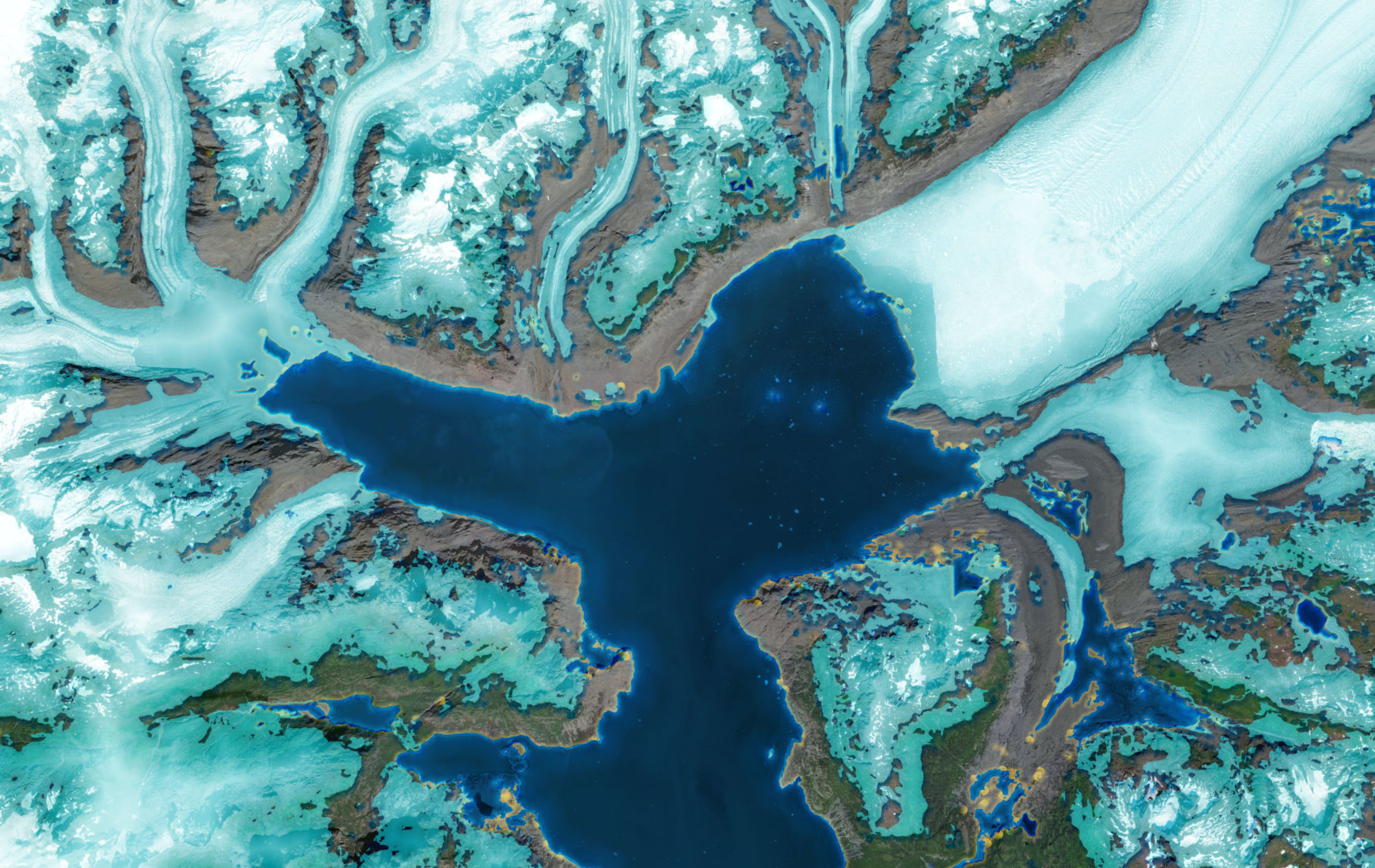
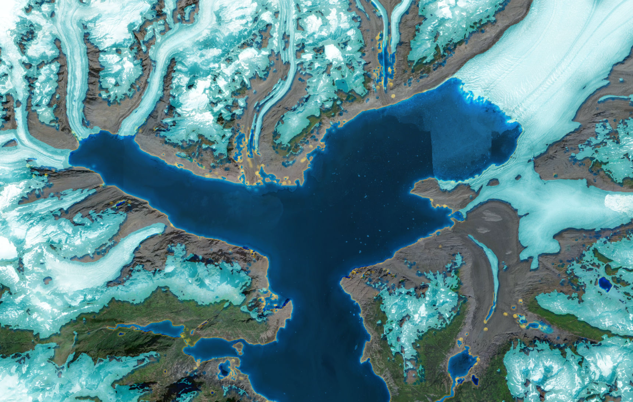
I made these two maps below using ArcGIS. The maps are of the same space but represent two periods of time, 2017 and 2022. These maps show a dramatic change in the size of a glacier in Alaska. To create this comparison I used ArcGIS’s land cover website and was able to choose two years to explore. After downloading the data, I was able to turn it into polygons. From there I seperated the data into ice and water polygons. I then sylized it too blend in with the base map.
Compare the two images: Click and slide the blue slider to observe the change over time:
I created the map below using ArcGIS. This was a fun project for me to work on and allowed me to practice stylistic map making that didn’t involve data. To create this, I added several layers and adjusted them to create a forced perspective. I was able to work with colors, gradients, hatched lines, filters, and shape and line effects to create a fun watercolor map.
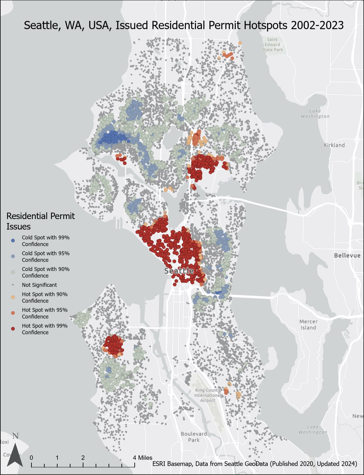
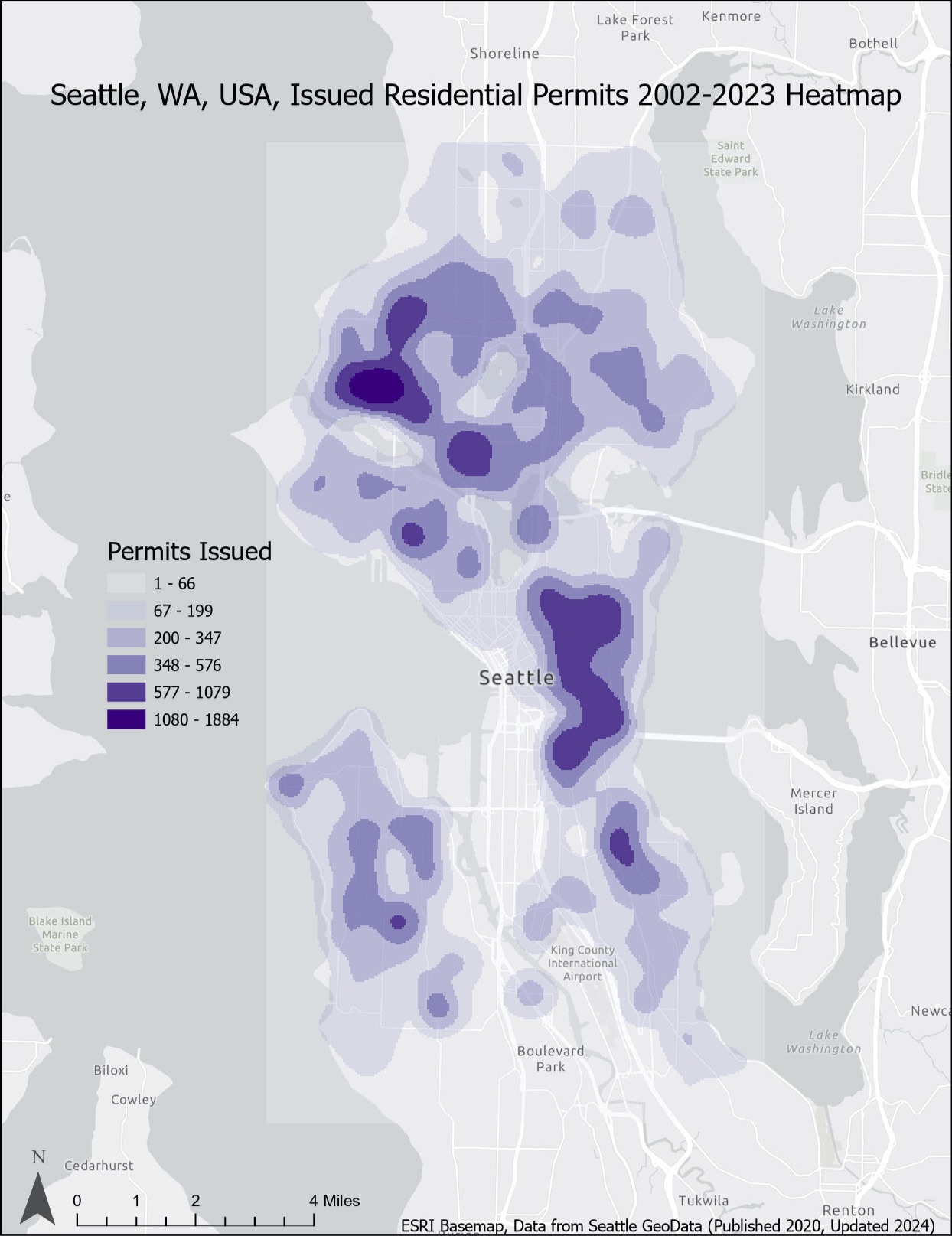
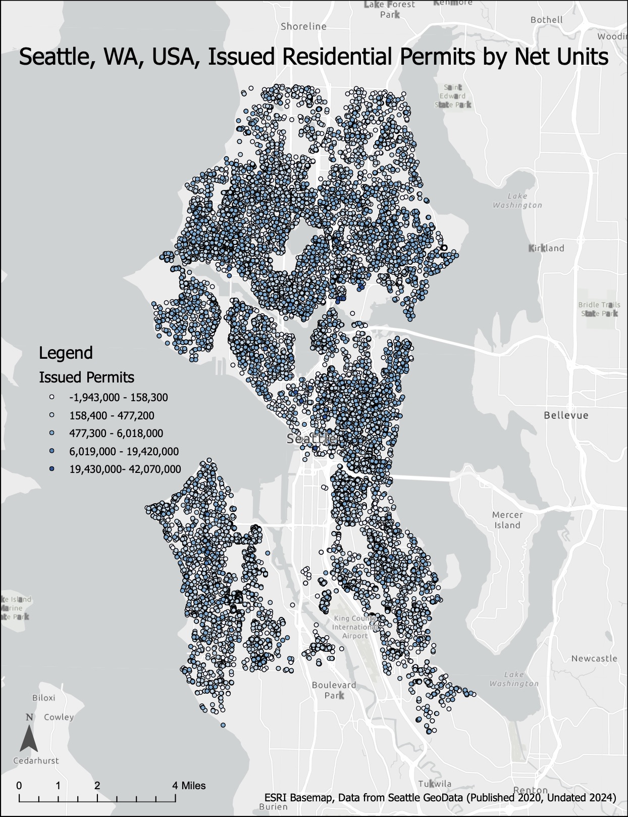
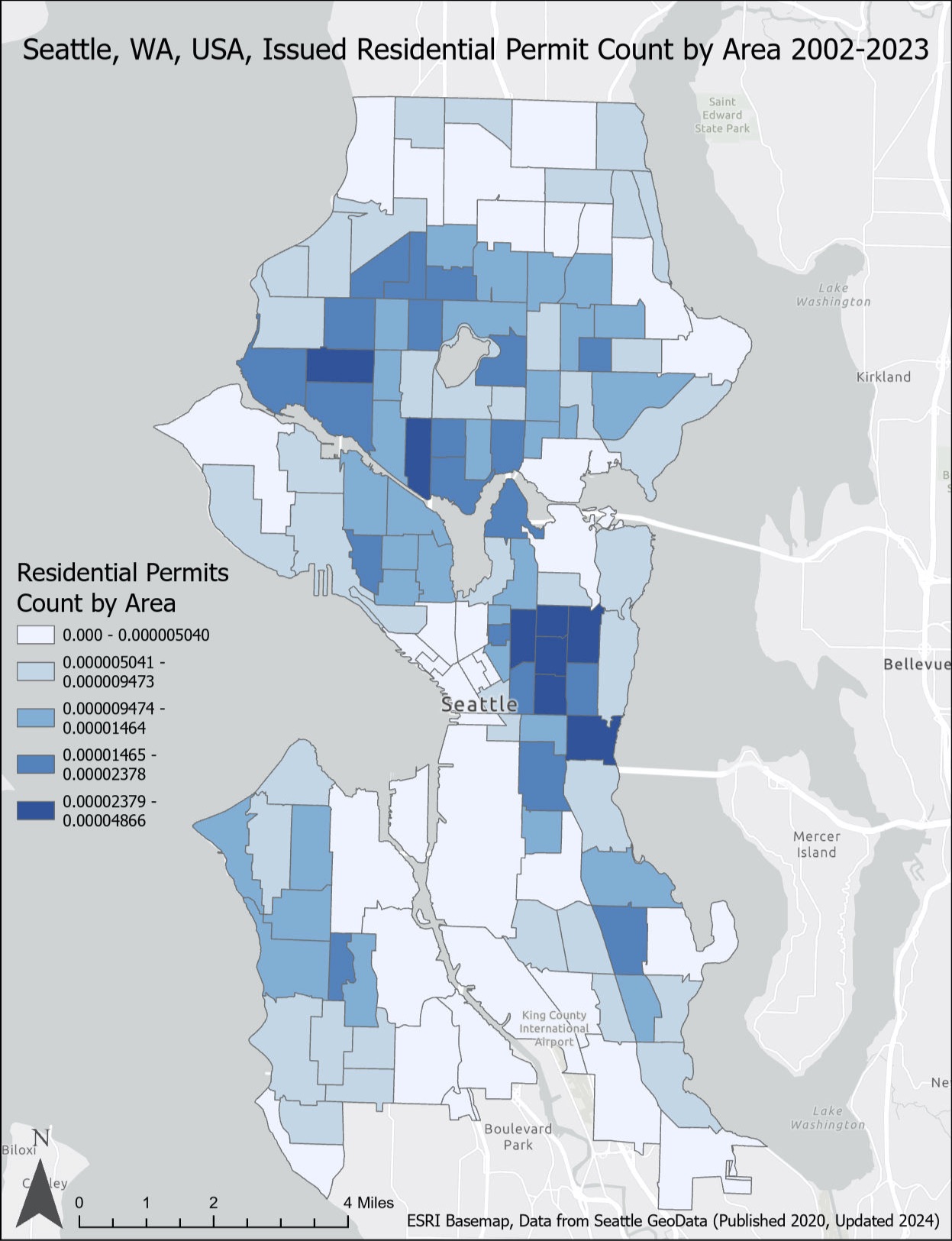
I created the maps below using ArcGIS. The data was found using Seattle GIS data to create multiple maps that represent different spatial patterns of issued residential construction/decontruction data. Some of the data is normalized based on the number of units in the area.
In the map below I used QGIS and raster data to predict mosquito presence in Kenya during the month May. In May, there is the most exposure to mosquitos, and in association, malaria. This map predicts which areas may be more riskey based on elevation and temperatures that mosquitos can survive in.
The map below was created using QGIS and depicts the number of people who live more than five miles from a voding dropbox in King County Washington. This map displays inequalities in access based on location.
The map below was created using QGIS and uses raster data that calculates historic temperature and predicted temperature to display locations that will be affected most by climate change. More information can be found in the description below the map.
This map was created using QGIS and depicts CO2 emissions by region compared to estimated population. More information can be found in the description below the map.
This Sankey Diagram was created using Google Colab. To create this visualization, I found data on Seattle interstate flow, cleaned the data, and visualized it. Each city is connected by a line, the size is proportional to the quantity of traffic flow.
This visualization was created using a Yelp web crawler, Observable, and QGIS. First I found eleven bars in Capital Hill, Seattle. I used web crawler to find comments, I then visualized it with using observable. I then created the central map on QGIS.
This visualization was created using R Studio. It represents the color of the sky from outside my apartments balcony throughout the day. Almost every ten minutes from 11:30am to 9:30pm I took a picture from my apartments balcony to create this visualization. Once the pictures were taken, I broke the photos down into their 10 primary colors and visulized them in the graph below.